The metrics¶

A continual-learning policy is not judged by one number. It is judged by how it behaves around change: how much it earns under each set of conditions, how quickly it finds its footing after conditions shift, whether it loses what it knew when earlier conditions return, how steadily it performs, and how far short of the achievable it settles. This chapter defines every number the package reports — formally, in plain language, and on a worked example small enough to recompute by hand.

Two rules hold throughout, because breaking either corrupts everything downstream:

An unavailable metric is absent, never zero. Zero is a value these metrics can take, so the tables print -- for absence and the library returns nothing rather than substituting.
Runs are segmented by the regime label, and by nothing else. Rollout windows are training administration; configuration intervals are what the protocol measures over.

Notation¶

Symbol	Meaning
\(r_t\)	the reward recorded at step \(t\)
\(z_t\)	the regime label recorded at step \(t\)
\(T_k\)	a configuration interval: a maximal run of steps with \(z_t = k\); \(T_k^{(1)}, T_k^{(2)}\) are the first and second such intervals
\(\bar r_\tau\)	the running mean over an interval's first \(\tau\) steps, \(\frac{1}{\tau}\sum_{i=1}^{\tau} r_i\)
\(\alpha\)	the adapted fraction (default \(0.9\) against a segment's peak, \(0.5\) against a ceiling)
\(\varepsilon\)	recovery's tolerance (an absolute distance under the ceiling anchor; a fraction, default \(0.30\), under the segment anchor)
\(R_{\mathrm{ub}}\)	the reward's theoretical ceiling, derived from its specification

The worked example¶

Thirty steps, three intervals. Regime a pays a steady \(0.8\); a shift to b finds the policy briefly lost (\(0.1\)), then over-corrected (\(0.9, 0.9\)), then settled at \(0.6\); a return to a's conditions — scheduled as a_again, an alias of a — now pays only \(0.5\). The block builds the trace and scores it; it runs when this documentation is built, and the output shown is the output produced.

from skyfall_crl.eval.metrics import EpisodeTrace, compute_all_metrics
from skyfall_crl.rewards.trace import EpisodeStep

rewards = [0.8] * 10 + [0.1, 0.9, 0.9] + [0.6] * 7 + [0.5] * 10
labels = ["a"] * 10 + ["b"] * 10 + ["a_again"] * 10
trace = EpisodeTrace(steps=[
    EpisodeStep(step=i, reward=rewards[i], regime_id=labels[i],
                regime_origin="a" if labels[i] == "a_again" else None)
    for i in range(30)
])
table = compute_all_metrics([trace])

for k in ("a", "b", "a_again"):
    row = table["per_regime"][k]
    fmt = lambda v, spec: "--" if v is None else format(v, spec)
    print(f"{k:<8} J = {fmt(row['per_configuration_reward'], '.4f')}"
          f"   adapt = {fmt(row['adaptation_speed'], '.0f')}"
          f"   recover = {fmt(row['recovery_time'], '.0f')}"
          f"   forget = {fmt(row['forgetting'], '+.4f')}"
          f"   variance = {fmt(row['stability_variance'], '.4f')}")

a        J = 0.8000   adapt = --   recover = --   forget = +0.3000   variance = 0.0000
b        J = 0.6100   adapt = 3   recover = 2   forget = --   variance = 0.0477
a_again  J = 0.5000   adapt = 1   recover = 1   forget = +0.3000   variance = 0.0000

Three absences in that table are correct, and the sections below explain each: a has no adaptation or recovery because no shift precedes the run's first interval, and b has no forgetting because its conditions never return. Note also that a's variance is \(0.0000\) — a value, earned by a perfectly steady reward, and exactly why absence must not be written as zero.

What adaptation and recovery are measured against¶

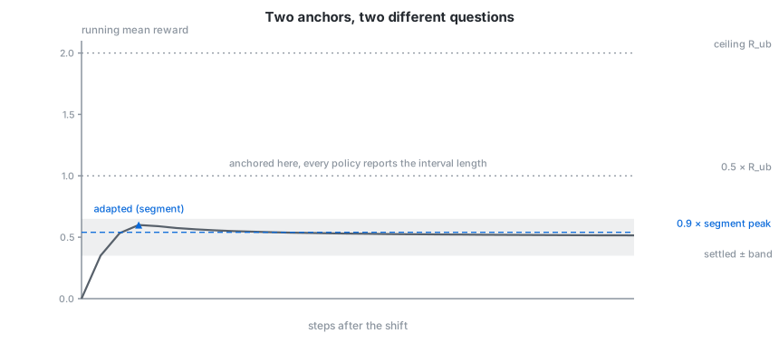
Both metrics compare a running mean to a reference, and the choice of reference — the anchor — changes the question being asked.

Two anchors, two different questions

Anchor	Reference	Default \(\alpha\)	The question
`segment` (default)	the interval's own behaviour — its peak running mean, its settled tail	\(0.9\)	how quickly did the policy get to where it was going?
`ceiling`	the theoretical bound \(R_{\mathrm{ub}}\)	\(0.5\)	how quickly did it reach a workable absolute level?

The ceiling anchor is the classical formulation, and it is the right one when the ceiling is attainable. When it is not — a bound assembled from maxima that never co-occur can sit orders of magnitude above any realistic reward — every policy fails to cross \(\alpha R_{\mathrm{ub}}\), every family reports the interval length, and the metric stops discriminating. The data-relative segment anchor is the default for that reason. The two anchors answer different questions, so a number computed under one is not comparable to a number computed under the other; every table records which anchor produced it.

The six¶

Per-configuration reward¶

\[ J_k \;=\; \operatorname{mean}\{\, r_t : z_t = k \,\} \]

The mean reward over every step recorded under label \(k\), pooling all of that label's intervals. Reads as: how good was the policy under these conditions, overall. In the example: \(J_a = 0.8\), \(J_b = 0.61\) (the ten b rewards sum to \(6.1\)), \(J_{a\_again} = 0.5\). Note that a and a_again report separately here — per-configuration reward segments by label, while forgetting (below) pairs them by identity. Pitfall: \(J\) is unanchored — comparable across configurations within a run, meaningless across environments with different reward scales.

Adaptation speed¶

Over the interval that begins at the shift, with running mean \(\bar r_\tau\):

\[ \tau_{\mathrm{adapt}} \;=\; \min\{\, \tau : \bar r_\tau \ge \alpha \cdot A \,\}, \qquad A = \begin{cases} \max_{\tau'} \bar r_{\tau'} & \text{segment anchor} \\ R_{\mathrm{ub}} & \text{ceiling anchor} \end{cases} \]

Reads as: how many steps after the change before the policy was most of the way to its eventual level (segment), or to a workable absolute level (ceiling). In the example, b's running means are \(0.1, 0.5, 0.6\overline{3}, 0.625, 0.62, \ldots\) — the peak is \(0.6\overline{3}\) at \(\tau = 3\), the threshold is \(0.9 \times 0.6\overline{3} = 0.57\), and the first running mean at or above it is \(\tau_{\mathrm{adapt}} = 3\). For a_again the running mean is constant at \(0.5\), so the threshold (\(0.45\)) is met at \(\tau = 1\): returning to known conditions costs one step, which is the backward-transfer story told as a speed. The two anchors disagree about "never": under the segment anchor a policy that never crosses reports the interval length \(|T_k|\) — by the end of its interval it is at its own peak by definition — while under the ceiling anchor it reports unavailable, because "never reached the level" is a finding, not a duration. Pitfall: the first interval of a run has no shift and reports nothing; a stationary run therefore has no adaptation speed at all.

Forgetting¶

\[ F_k \;=\; \operatorname{mean}\!\big(T_k^{(1)}\big) \;-\; \operatorname{mean}\!\big(T_k^{(2)}\big) \]

Positive means the policy got worse. The two encounters are paired through the regime's origin, so a revisit scheduled under a fresh label — a_again, an alias_of a — still counts, and both labels report the same number.

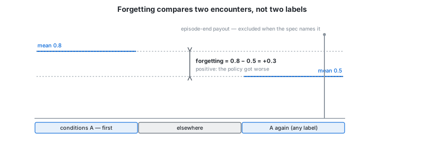
Forgetting compares two encounters, not two labels

In the example: \(F_a = 0.8 - 0.5 = +0.3\) — the policy returned to a's conditions earning less than it did the first time. That is forgetting. A negative value is backward transfer: the return went better, usually because something learned in between generalised. Pitfalls: it needs a recurrence — a schedule that never returns to anything reports --, which is why schedules built to measure forgetting carry an alias entry. An earlier implementation of the same name computed the difference the other way around, so a number carried across analyses inverts its sign; check the convention before comparing. And when a reward has episode-end terms, the payout typically lands in the second encounter — name those components and the affected steps are excluded, so forgetting is not decided by which interval contained an episode's end.

Recovery time¶

Under the segment anchor, with asymptote \(A\) = the mean of the interval's final \(\lceil 0.2\,|T_k| \rceil\) rewards:

\[ \tau_{\mathrm{rec}} \;=\; \min\Big\{\, \tau : \big|\, \bar r_\tau - A \,\big| \;\le\; \max\big(\varepsilon \cdot |A|,\; 0.005\big) \Big\} \]

Reads as: how many steps until performance settled — near its eventual level, from either side — as opposed to adaptation's reached — a threshold, from below. The absolute floor (\(0.005\)) is load-bearing: without it a settled state at or near zero has a zero-width band and the metric can never trigger. In the example, b settles at \(A = 0.6\) (the mean of its last two rewards), the band is \(\pm 0.18\), and the running mean enters it at \(\tau_{\mathrm{rec}} = 2\) (\(|0.5 - 0.6| \le 0.18\)) — before adaptation, legitimately: the running mean was already near its settling point while still short of its peak. Recovery genuinely failing to trigger reports --. Pitfall: under the ceiling anchor with default tolerance (\(\varepsilon = 0.5\,R_{\mathrm{ub}}\)), recovery asks nearly the same question as adaptation — any mean below \(1.5\,R_{\mathrm{ub}}\) satisfies both at once — which is why published tables show a recovery of exactly \(1\) wherever adaptation was fast.

Stability¶

\[ \sigma^2_k \;=\; \operatorname{Var}\{\, r_t : z_t = k \,\} \]

Reward variance within a configuration — reported pooled across the label's intervals, and per interval. Reads as: how steady the policy is once conditions hold still; between two policies with equal \(J_k\), the lower-variance one is the one to deploy. In the example, \(\sigma^2_b = 0.0477\) — the price of the \(0.1\) stumble and the \(0.9\) over-correction — while both a intervals report exactly \(0.0\), steadiness so perfect it illustrates the absence rule: a single-step interval would report --, not \(0.0\), because one sample has no variance. Pitfall: variance does not distinguish exploration from instability; read it beside the trace.

Performance gap¶

\[ \Delta_k \;=\; R_{\mathrm{ub},k} \;-\; \operatorname{mean}\big(\text{final } 20\% \text{ of } T_k^{(1)}\big) \]

How far the settled state falls short of the ceiling. Reads as: the improvement still on the table under these conditions. It is the one metric that requires a ceiling, so without a specification or an explicit bound it reports --. Pitfall: when the ceiling is a sum of maxima no policy could earn at once, the gap mostly restates the ceiling — report the settled reward alongside it (below), which carries the same information without the subtraction.

The ceiling¶

\(R_{\mathrm{ub}}\) is derived, not asserted. Because every component of a reward specification declares a clip and a weight, the most each term can contribute is known from the specification alone, and the analytic bound is their sum — computed separately for an ordinary step and for an episode's final step, since EPISODE_END terms can only pay there:

from skyfall_crl.eval.upper_bound import analytic_upper_bound
from skyfall_crl.rewards import get_spec

for name in ("paper", "experiment"):
    bound = analytic_upper_bound(get_spec(name))
    print(f"{name:<12} per step {bound.per_step:.4f}   final step {bound.final_step:.4f}")
bound = analytic_upper_bound(get_spec("experiment"))
print(f"interval of 60 holding the final step: "
      f"{bound.for_interval(60, contains_final_step=True):.4f}")

paper        per step 0.0000   final step 0.5000
experiment   per step 0.3333   final step 1.0000
interval of 60 holding the final step: 0.3444

A paper step's ceiling of \(0.0\) is informative, not broken: that specification's only per-step term is a pure penalty, so the best an ordinary step can do is nothing. The interval form \(\big((L-1)\,p + f\big)/L\) is what a configuration interval is actually measured against, since the metrics compare means. Two more derivations exist for rewards the closed form cannot bound: a numeric estimate (drive the composition over supplied contexts and take the best achieved) for specifications with unclipped components, and a data-relative bound (the best observed in recorded traces) — useful, but derived from the policy being measured, so two policies compared against their own data-relative bounds are not being compared fairly. Every result records which derivation produced its bound.

Everything the table prints¶

skyfall-crl eval renders fifteen rows. The six above, then:

Row	Definition	`--` when
Zero-shot reward	mean reward over the first 10 steps after a shift — performance before adaptation	no shift in the trace
Regret	\(\sum_t (r^{\mathrm{ref}}_t - r_t)\) against a supplied reference trajectory	no reference supplied — the protocol is deliberately oracle-free
Effective rank	mean of the recorded per-step effective rank of the policy's representation — a plasticity reading; falling rank with flat reward is a policy losing the capacity to learn	the run never measured it (capture is off by default)
Settled reward	the tail mean itself: mean over the final 20% of each interval, averaged across intervals — the value whose distance the performance gap reports	the label never ran
Settled reward (policy)	the same, excluding steps that carried an episode-end payout — the part the policy earned in-conditions	no episode-end components named
Return (discounted)	\(\sum_t \gamma^{\,t}\, r_t\) over the whole trace (\(\gamma = 0.99\) by default)	—
Return (undiscounted)	\(\sum_t r_t\)	—
Invalid-action rate	fraction of steps whose action the environment refused	—
Solve rate	fraction of steps on which a named reward component was positive — "a unit of work completed"; the component's name belongs to the environment, so it must be given	no component named

One more is computed between runs rather than within one: relative adaptation advantage, \(\tau_{\mathrm{adapt}}^{\mathrm{baseline}} - \tau_{\mathrm{adapt}}^{\mathrm{self}}\) — positive means faster than the baseline family. It appears in cross-family comparisons, where each side is a family's mean across seeds.

How numbers aggregate¶

Within one result, aggregation is two-stage: a metric is averaged across traces within a configuration, then across configurations — with absences dropped at both stages, never counted as zero. Comparing families adds a third stage: each family's per-seed results aggregate to a mean and a spread across seeds, and a family with one seed reports no spread rather than a zero one. Every stage preserves the absence rule, which is why a -- in a final table can be trusted to mean unmeasured rather than zero.

Reading the numbers without being misled¶

-- is not zero. A column of absences means the question could not be asked — no shift, no recurrence, no ceiling — not that the answer was nothing.
A stationary run answers almost nothing. One regime for the whole run gives \(J\) and variance; adaptation, recovery, forgetting and zero-shot all need change.
A spread of exactly zero across seeds usually means the seeds reached nothing. If every seeded run is identical, the seed varied nothing that mattered — check what the seed was actually wired to before reading the spread as certainty.
Anchors do not mix. A segment-anchored adaptation speed and a ceiling-anchored one are answers to different questions; tables record the anchor precisely so numbers are not carried between them.
Near-noise rewards differentiate in late decimals. When realistic per-step rewards are small, families can differ in the third or fourth decimal place; the spread across seeds, not the mean alone, says whether such a difference is real.
Pooled intervals can hide structure. \(J_k\) pools every interval of a label; when a revisit behaves differently from a first encounter, the per-interval view (and forgetting) carries the story the pooled mean averages away.